

Smart glasses production capacity is the kind of number that is easy to describe and hard to plan against, and the fastest way to understand what makes it plannable is to watch one fail. This is a hypothetical case rather than a client project: the buyer, the quantity, the market and the dates are constructed to illustrate a method, and none of them describe a real order. What the example demonstrates is the sequence of decisions that turns a quoted rate into a schedule that closes, and the point at which the plan stops closing and has to be changed. It is written for the brand-side procurement manager, the channel buyer and the importer who has a launch date and a quantity and needs to know whether the two can live together. The production capacity assessment section covers the same method from the supply side, and the sample evaluation section covers the approval step that sits between the quotation and the plan.
A worked smart glasses production capacity plan, start to finish
The hypothetical programme, and why it is stated this way
The constructed programme is a European channel launch of three camera configurations, ordered as one programme and delivered as one consignment. The three are chosen because they are genuinely different builds rather than three colourways of one: a magnetic-charged eight-megapixel entry with a removable inner frame and an IP54 marking, a magnetic-charged thirteen-megapixel entry with the same removable frame and IP54 marking, and an eight-megapixel entry that ships with a folding charging case of twelve hundred milliamp-hour capacity. The first two are published in the catalogue with a two-hundred-and-sixty milliamp-hour cell and a five-to-eight-hour runtime; the third is published with a two-hundred-and-sixty-five milliamp-hour cell and a runtime of about seven hours, and it is the only model in the range with a published weight, one hundred and fifty-eight grams for the glasses themselves, excluding the folding case.
That mix matters because the three builds do not consume the same effort. Two are magnetic-charged, one is not, and the published catalogue does not record a charging method for four of the eleven camera entries at all, which means the charging route for a camera build is a question a buyer has to ask rather than a specification they can assume. The three also sit at two different resolution tiers, and the resolution tier is one of the reasons a test step is not a constant across the range.
The quantities are constructed as well, and they are deliberately unbalanced: forty thousand units of the first configuration, sixteen thousand of the second and four thousand of the third. Total sixty thousand. The imbalance is realistic, because the configuration a buyer launches with is normally the one with the simplest supply position, and the one added later is normally the one with the longest lead.
The assumptions the walkthrough starts from
Five assumptions carry the example, and they are stated up front because a worked example that hides its assumptions teaches the wrong lesson.
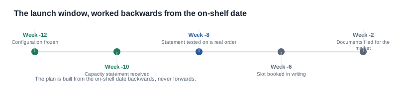
The on-shelf date is fixed. The channel has already committed to a launch window, and the goods have to be in the seller's warehouse four weeks before that window opens, which puts the whole working period at twelve weeks from the configuration freeze to the on-shelf date.
The order is one consignment. No split shipment, no partial delivery, because a split changes the logistics arithmetic and the customs position and would obscure the point the example is making.
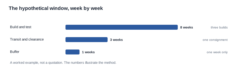
The build window is eight weeks. Twelve weeks less two weeks of transit and less one week of buffer leaves eight weeks of build and test, which at six working days a week is forty-eight working days.
The supplier quotes a range, not a figure. Between nine hundred and fourteen hundred units a day for the camera range, with a stated basis of lines, shifts and cycle time, and with a committed load that takes one line out of the building for the second half of the month.
The release rate is asked for separately. The buyer does not accept the build rate as the answer, because a dispatch date depends on units that are finished, tested, packed and cleared rather than units that are assembled.
With those five in place, the required rate can be calculated. Sixty thousand units over forty-eight working days is one thousand two hundred and fifty units a day. The quoted range runs from nine hundred to fourteen hundred. The buyer's requirement sits between the middle and the top of it, which is the first thing the plan has to survive.

Building the window backwards from the on-shelf date
What the arithmetic says about the low end
The planning figure is the low end of the range, because a programme that plans to the middle is planning to a number nobody measured. At nine hundred units a day, forty-eight working days produce forty-three thousand two hundred units. The requirement is sixty thousand. The shortfall is sixteen thousand eight hundred units, which is close to a quarter of the order.
The middle of the range does not save the plan either. At roughly one thousand one hundred and fifty units a day the window produces fifty-five thousand two hundred units, which is still short. Only a rate at or above one thousand two hundred and fifty closes the window, and that rate sits in the top third of the quoted range, above its midpoint. A plan that closes only when the factory delivers near the top of its own range is not a plan; it is a forecast with the word plan attached.
This is the first lesson of the example, and it is a lesson about the shape of the answer rather than about the factory. A quoted range is not a plan, and a required rate that lands in the upper third of a quoted range is a warning that the plan will be built on hope.
The release rate, and where the shortfall really lives
What follows is to ask for the release rate inside the quoted range, and this is where the shortfall becomes explicable. On the built configuration, a meaningful part of the working day is consumed by the test step, by the case assembly on the entry that ships with a folding case, and by the queue in front of the release bench. The release rate therefore sits below the build rate, and the gap is not a rounding error.
The practical consequence is that the sixteen thousand eight hundred unit shortfall is not a factory-capacity problem. The factory may well have the lines. The problem is that the lines, the test benches and the release window together cannot move sixty thousand units through a forty-eight day window, and the arithmetic that closes the plan has to include the release step, not just the assembly step.
The three decisions that set the outcome
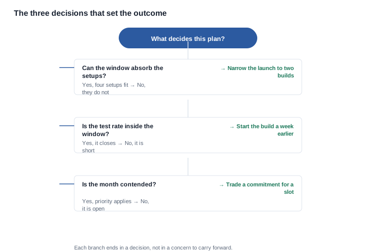
At this point the example has three options, and each one changes something the buyer cares about differently.
Narrow the first wave. Move the thirteen-megapixel configuration out of the launch and into a second wave. The first wave becomes forty-four thousand units, which at nine hundred units a day over forty-eight days is comfortably inside the range's low end, with the configuration set reduced and the setup burden cut at the same time. The cost is that the launch has no thirteen-megapixel option on the shelf in the first window, and the channel that was built around a broad opening loses part of its range.
Start the build earlier. Take the one-week buffer out of the window and extend the build to nine weeks, fifty-four working days. Forty-four thousand units at nine hundred a day closes comfortably, and the sixty-thousand-unit first wave also closes at a rate of one thousand one hundred and eleven a day, which is inside the range. The cost is that the buffer is gone, and every subsequent delay lands directly on the on-shelf date.
Split the order. Two consignments, the larger configurations first, which lets the programme start selling before the whole order exists. The cost is the one the example assumed away at the start: a split changes the logistics, the clearance and the way the shortage lands if the second shipment is the one that is late.
In the constructed example the buyer takes the first option and the second together, which is the usual shape of the answer: narrow the first wave, and start a week earlier to keep some buffer. The result is a plan that closes at the low end of the quoted range with two weeks of slack rather than one.

Testing the plan against a real order
Where the statement held and where it did not
The corrected plan is then run against a real order, because that is the step that catches a number nobody thought to check. The buyer takes the most recent order of similar size it has placed with this supplier, substitutes the new configuration set and the new build window, and runs the supplier's own stated figures against it.
Two things come out. The first is that the stated daily rate holds for a single configuration running over a long window, which is what the basis suggested, and the figure is therefore usable. The second is that the four configuration changes in the first wave were not in the rate the supplier quoted, because the rate was quoted for one configuration at a time. Each changeover costs time that produces no saleable units, and four of them inside a forty-eight day window is a material deduction rather than a rounding.
This is the point at which a plan built on the quoted range stops matching the plan that will actually run, and it is exactly the point a formal test is meant to find. The correction is to have the changeover time stated for the specific build sequence, which is a question a supplier can answer and which the original quotation did not raise.
The questions to ask, in the order the example asked them
The walkthrough is only useful if the buyer can repeat it, so the questions are listed here in the order they were actually asked. The order is what made the answers build on each other, and it is the reason the same supplier can be compared with another one afterwards.
- What is the build window, worked backwards from the date the goods have to be in stock?
- What is the required daily rate for that window, once the configuration set is fixed?
- What is the rate you would quote, with its unit, its period, its basis and its derivation?
- What is the release rate inside that range, for this configuration, on these lines?
- Which purchased parts could cap the output below it, and what are their lead times?
- What is the committed load on those lines in the build month?
- How long is a changeover for this build sequence, and what is the longest run length?
- What is the slot in a contended month, and what is the priority rule?
- What was the rate on the last comparable order, and did it hold?
Before you order, question nine is the one that converts the whole exercise from arithmetic into evidence, and question seven is the one most often skipped. A buyer who has the changeover time in the file before the order is placed can cost a post-freeze configuration change; a buyer who does not has to accept it.
The criteria these nine questions satisfy are worth stating, because they are what the example was testing throughout: a rate that is reproducible from its basis, a release rate that is separate from it, a named parts exposure, a named load, a stated changeover, a written slot, and a record of what actually happened last time. If a supplier answers all nine in writing, the buyer's remaining work is narrow and arithmetic. If they answer two, the buyer has a capability description and a decision to make about how much risk to carry.
The correction, and what it cost
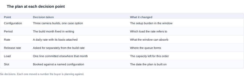
After the changeover is stated, the window is re-planned with the four configuration changes inside it rather than assumed away, and the resulting plan gives the buyer a figure it can commit to: the first wave of forty-four thousand units, built across four configuration changes, closing inside forty-eight working days at the low end of the quoted range.
The cost of the corrections is worth stating plainly because procurement reports tend to record only the outcome. The launch lost its thirteen-megapixel option for one window, which is a commercial decision with a price attached and a marketing consequence. The plan ran on a one-week buffer instead of two, which reduced the programme's ability to absorb a further delay. And the supplier's commitment became specific in a way it had not been, which is a gain and also a constraint: the order now depends on a release rate and a changeover time that have been written down and can be checked, and it depends on a parts position that has been named.
The last point is where the example connects to supply chain risk. The quoted rate assumed that the camera modules, the cells and the folding cases for the third configuration would arrive in time. The buyer asked which parts could cap the output, and got a named list with lead times, and the third configuration was the one with the longest exposure because the folding case is a bought item with a single source. That is the condition the buyer carried forward, and it is the condition that would have broken the plan.

The breakpoints that would have broken the plan
Four named breakpoints
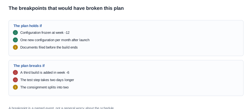
A plan is not robust because it has a buffer. It is robust because the things that would break it have been named, and each named breakpoint has an owner and a response.
A third configuration added in week six. The launch was already frozen, and a new configuration inside the build window adds a changeover that was not costed and a parts demand that was not on order. The response is a change control point with a date, and a rule that a post-freeze change carries a visible schedule cost.
The test step running two days longer than stated. On a forty-eight day window, two days is four per cent of the window, and it comes out of the buffer before anything else. The response is a weekly release-rate check against the plan, which is a cheap control with an early signal.
The consignment splitting into two. A split is not a logistics inconvenience here; it is a change to the customs position and the way a shortage is experienced by the channel. The response is to decide the split rule in advance rather than discovering it.
The folding case arriving late for the third configuration. The lowest-volume configuration in the example carries the longest exposure, because the case is a bought item with a single source. The response is to ask for the part lead time in writing and to hold the configuration's start date at the point the part is actually available rather than at the point the plan wanted it.
The one that was most likely
Of the four, the one most likely to occur is the simplest: a configuration change after the freeze, and the reason is that the configuration freeze is a commercial decision while the change is usually a commercial request. A channel asks for a colour or a case option in week six, and the request is reasonable and small, and accepting it costs a changeover that nobody priced.
The example's plan handled this by making the post-freeze change visible before it was made rather than by prohibiting it. That is the same discipline that applies to the launch date, the documentation route and the AI camera glasses range options: a change that carries a stated cost is a change that gets decided, and a change that costs nothing on paper is a change that gets assumed.
What the walkthrough teaches, and what we publish
The method the example demonstrates
Five things carried the example from a quoted range to a plan that closes, and they are worth repeating because they are the whole method. Work backwards from the date the goods have to be in stock. Convert the requirement into a daily rate before comparing it with anything. Plan to the low end of the range, not the middle. Ask for the release rate and the changeover time separately from the build rate, because both of them sit between the quoted figure and the delivered goods. And test the result against a real order before the order is placed.
The example also shows what a plan is not. It is not a quotation with a date attached, and it is not a rate with a window drawn around it. It is a specific set of decisions about configuration, volume, window and sequencing, each of which changes a number the buyer is planning against, and each of which can be revisited when something moves.
The commercial terms the plan produces
A plan of this shape is also the only sensible basis for negotiating, because it converts a general claim into a set of specific ones. What to ask for and what to concede both follow from the walkthrough. The priority rule, the release rate, the changeover time and the named parts exposure are all things the supplier can now commit to, because the buyer has done the arithmetic that makes them meaningful. In return, the buyer has something the supplier wants: a frozen configuration, a firm quantity and a window that is realistic rather than optimistic.
The trade-offs are the usual ones, and the example makes them concrete. A narrower first wave buys schedule certainty and costs range breadth on the shelf. A firm volume commitment buys a better slot and costs the buyer flexibility when the channel's demand moves. An earlier build start buys a buffer and costs working capital. The total cost of the arrangement is the unit price plus the returns reserve plus the documentation route plus the inventory held against a schedule the buyer does not control, and in a case like this the last of those is usually the largest number in the model. The pitfalls worth naming are the ones the example already found: a rate quoted for one configuration and applied to three, a changeover that was never in the quote, and a parts exposure that was discovered late.
A buyer who wants to know how to evaluate the plan rather than how to defend it should go back to the nine questions above and ask them of a second supplier in the same order. How to compare two factories is not a matter of which of them sounded more confident; it is a matter of which of them produced answers that close.
The rate comes with a derivation, a release rate, and a changeover
We will produce a rate with its unit, its period, its derivation, its release rate and its changeover assumption for a named configuration, month and quantity, and we will show the line count, the shift pattern and the cycle time behind it. We will name the purchased parts that could cap the output, with the lead time on each, and we will state the committed load in the build month, because a rate quoted without a load is not usable.
We will not publish a standing daily output figure, a line count, a shift pattern, a defect rate, a rework rate or a capacity number for the range as a whole, and we will not quote one to a buyer who has not fixed a configuration and a month. All of them are functions of the mix and the current order book, so a published figure would be true for a configuration that does not exist and misleading for the one that does. We will not quote a typical range, and we will not write a figure into a plan that cannot be traced back to a record.
What we do is take a programme of this shape and return the plan that belongs with it: the build window worked back from the date the goods have to be in stock, the rate with its derivation, the release rate, the changeover assumption for the build sequence, and the parts that could cap the output. Every one of those numbers carries the condition it depends on, which is what makes the plan usable in a schedule rather than merely reassuring. The logistics section covers the part of the plan that sits after the build.
Related reading
Send the configuration, the quantity and the month, and we will return the plan with the assumptions written into it.